Deployment Diagrams

Deployment diagrams are useful at all stages of development. They provide a physical view of the system, and show the files and the devices they run on. In particular, they show:

• the coarse structure of a system
• which devices are involved
• how devices are connected to each other
• which devices run which software

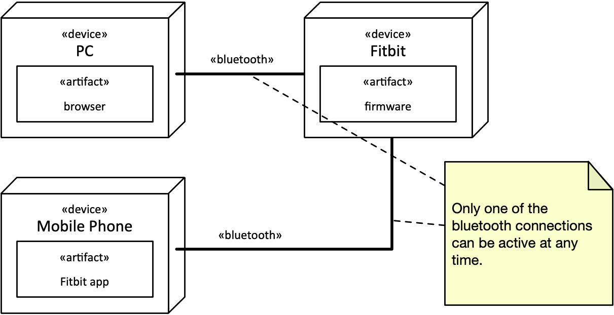
Below is an example for a deployment diagram, showing the elements of a fitness tracker (here a Fitbit) and how it works together with a mobile phone and the server backend.

What can we learn from this diagram?

• To the left, there is the Fitbit server, which is connected via HTTPS to a PC and the mobile phone of a user.
• On the PC, a browser is running.
• On the mobile phone, we have an application.
• The Fitbit is connected to PC and mobile phone via Bluetooth.

When we apply some color, we can see that deployment diagrams basically consist of three types of modeling elements:

1. Nodes that represent hardware devices and software execution environments (in blue). In other words, locations in the system that can execute software.
2. Connections that represent communication between nodes (in red).
3. Software artifacts that are assigned to nodes (in yellow).

Nodes: Devices

Devices are shown as a 3D-box with «device» printed at its top. The funny brackets are called guillemets and are each a single character. This is a notation for stereotypes, which are a kind of marker in UML.

Examples for devices are:

• PC
• Raspberry Pi
• Mobile Phone
• Tablet
• iPhone
• server
• gateway
• ...

These device types are not built into UML, you can decide on your own. Which ones make sense depends on your project. Is it relevant and informative that you are talking about a Raspberry Pi? If yes, fine! If it doesn't matter, use a more generic device type.

Nodes: Execution Environments

Software does often not directly run on hardware, but on some execution environment. If you want to show this, you can use a node (again with 3D effect) and the stereotype «execution environment».

Examples for execution environments are runtime environment, application server, web server, operating system, Java virtual machine (JVM) or a container system like Docker.

Nested Nodes

In some cases it makes sense to show nested nodes.

You can show a device inside a device, for instance when you want to show a disk inside a PC or a trusted computation element in a phone. Other hardware elements within a device can be memory. You should only show such elements if there is something special you want to point out. Like a special type of memory that is critical for the system, or the trusted computation element that enables new use cases.

Usually, execution environment are contained within devices, since software needs to run on some hardware. The only reason not to show a device and have an execution as its own top-level element is when the hardware it necessarily runs on is obvious from the context or not important at all. One thing is sure, however: execution environments cannot contain devices.

In some cases, you might want to points out that an execution environment is nested inside another execution environment, like when you want to point out that Python runs within Docker, in a Linux operating system on a server. Again---assess for your specific case which information is relevant.

Showing Node Instances

Sometimes you want to show several nodes of the same type, but want to express that these are different instances. Example, an airport gate with several passenger turnstiles, that are physical identical. For that, you just include the instance name in front of a colon, like t1: Turnstile. In addition, you underline to make clear that you refer to a specific instance.

Communication Paths

When two nodes communicate, they are connected by a solid line. This line can be labelled with a stereotype that says something about the way of communication, by referring to a standard or a protocol, as for instance:

• «http»
• «mqtt»
• «amqp»
• «tcp/ip» or «tcp»
• «bluetooth»
• «CoAP»

Artifacts

The software itself that runs on hardware and inside execution environments comes in the form of artifacts. They are shown as simple rectangles, with «artifact» written at the top. They can represent any artifact we find in software, for example:

• Database
• firmware
• device driver
• configuration files (.xml, .txt, .properties,...)
• source files (.java, .py, .c)
• library files (.dll, .jar)
• executable files (.exe, .jar, .c)

Deploying Artifacts

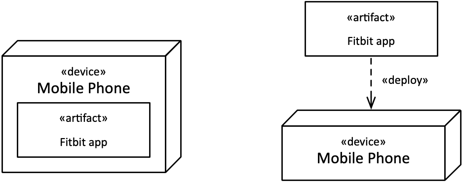
Software artifacts run within an execution environment or directly in a hardware nodes. There are two ways to assign a software artifact into a node:

1. Simply by drawing it into the node, that means, graphically by nesting.
2. By connecting them with a dashed line arrow labelled «deploy»

Below you see the two ways of deploying an artifact into a node. Both are semantically equivalent (they mean the same thing), but the graphics are different. Depending on how many artifacts to deploy and other layout constraints, either of them can be more compact and practical to use.

Manifestation

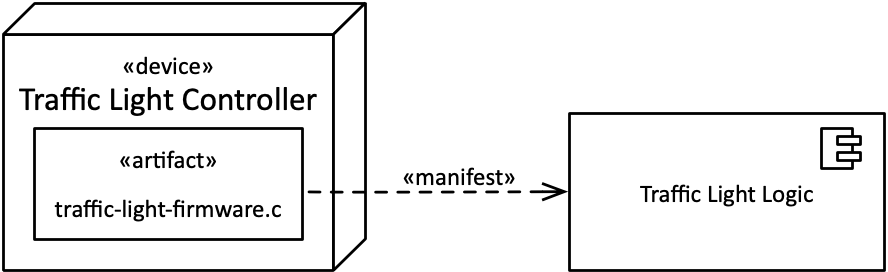
The software in an artifact can itself represent something we have modeled, like a UML component. This means that an artifact manifests other modeling elements.

In the example below, we show that the UML component Traffic Light Logic is manifested by the artifact traffic-light-firmware.c, using a dashed arrow with the stereotype «manifest». This means that there is a UML description of a traffic light encapsulated by the component Traffic Light Logic. This can be for example a state machine that describes in which sequences the traffic light cycles through red, yellow and green. (We will work with state machines later.) The state machines and the component, however, are only descriptions but cannot be executed on their own. For that, we need the code provided here by the artifact traffic-light-firmware.c, which implements for instance the component and state machines for the traffic light.

Hint: The difference between artifacts and nodes may appear subtle in some cases. Nodes that are devices describe physical pieces of hardware that you can touch. Artifacts, on the other side are often files, like source files or executable files for a program. They are real, but you cannot touch them. Execution environments, which are nodes, are a bit more subtle. You cannot touch them, but they provide a place of executing software, which comes in the form of artifacts.

Notes

Similar to comments and documentation in source code, UML diagrams can contain notes. They can capture additional information that cannot be expressed by other elements.

Multiplicities

In some cases we can add useful information to the deployment diagram by showing how many instances of a pair of nodes are connected with each other.

A multiplicity specification is a tuple in the form n..m where n denotes the lower bound and m the upper one. (This implies that n is smaller than m.) To keep the upper value unbounded, we use the asterisk *. This leads to the following possible combinations in practice:

 

Multiplicity	Shorthand	Meaning
n..m		Minimum n elements, maximum m. (m>n)
0..1		optional value
1..1	1	exactly one
0..*	*	any number of elements, "many"
n..*		n or more
n..n	n	exactly n

The first column shows the multiplicity in n..m format. The second columns shows an equivalent shorthand notation if there is one, and the third column how the multiplicity it to be understood or pronounced in words.

We can use these multiplicities at both sides of a connection between nodes. If no multiplicity is specified, it means *, which implies many.

In most practical cases, you don't need to worry much about the multiplicities because they are often implicitly clear from the context. But in some cases you can emphasize details that you consider important. Typical examples are:

• One Fitbit only can sync with a single mobile phone, emphasized by a one-to-one relationship.
• One server is connected to many gateways.

If the number varies at runtime, use 0..* or * in short, just implying many.

Containment

We have seen above that some nodes in a deployment diagram can contain other nodes, depending on the node types.

The following containments are typical:

• An execution environment can run in a device.
• An artifact is deployed in a device.
• An artifact is deployed in an execution environment.

The following containments are also possible, but maybe less common. Use them if you want to show a detail that is important to point out, and consider if that makes sense.

• A device can contain a device. For instance, a computer (device) can contain a harddisk.
• An execution environment can contain another execution environment. For instance, a virtual operating system container could rund a Python runtime.
• An artifact could be composite, like a file stored in an archive.

The following combinations make no sense:

• An execution environment cannot contain a device.
• An artifact cannot contain a device.
• An artifact cannot contain an execution environment.

Overview of Elements

• Communication Path
  • «TCP/IP»
  • «MQTT»
  • «AMQP»
  • «RMI»
  • «CoAP»
• Nodes
  • «execution environment»
    • «application server»
    • «web server»
    • «operating system»
  • «device»
    • «server»
    • «gateway»
    • «desktop PC»
• «artifact»
  • «data base»
  • «firmware»
  • «device driver»
  • configuration files
    • .txt
    • .properties
    • .xml
  • source files
    • .cpp
    • .c
    • .py
    • .java
  • library files
    • .dll
    • .jar
  • executable files
    • .exe
    • .jar